> ## Documentation Index
> Fetch the complete documentation index at: https://wb-21fd5541-sdk-testing-latest.mintlify.site/llms.txt
> Use this file to discover all available pages before exploring further.
# Scikit-Learn
> W&B を使用して、実験管理とプロットの自動ログ記録により、scikit-learn モデルのパフォーマンスを可視化・比較します。
wandb を使えば、わずか数行のコードで scikit-learn モデルのパフォーマンスを可視化して比較できます。[例を試す →](https://wandb.me/scikit-colab)
## はじめに
### サインアップしてAPIキーを発行する
APIキーは、お使いのマシンをW\&Bに認証するために使用します。APIキーはユーザープロフィールから発行できます。
より手早く行うには、[User Settings](https://wandb.ai/settings) にアクセスしてAPIキーを作成してください。APIキーはすぐにコピーし、パスワードマネージャーなどの安全な場所に保存してください。
1. 右上にあるユーザープロフィールアイコンをクリックします。
2. **User Settings** を選択し、**API Keys** セクションまでスクロールします。
### `wandb` ライブラリをインストールしてログインする
`wandb` ライブラリをローカルにインストールしてログインするには、次の手順を実行します。
1. `WANDB_API_KEY` の[環境変数](/ja/models/track/environment-variables/)に APIキー を設定します。
```bash theme={null}
export WANDB_API_KEY=
```
2. `wandb` ライブラリをインストールし、ログインします。
```shell theme={null}
pip install wandb
wandb login
```
```bash theme={null}
pip install wandb
```
```python theme={null}
import wandb
wandb.login()
```
```notebook theme={null}
!pip install wandb
import wandb
wandb.login()
```
### メトリクスをログする
```python theme={null}
import wandb
wandb.init(project="visualize-sklearn") as run:
y_pred = clf.predict(X_test)
accuracy = sklearn.metrics.accuracy_score(y_true, y_pred)
# 時系列でメトリクスをログする場合は、run.log を使用する
run.log({"accuracy": accuracy})
# または、トレーニング終了時に最終メトリクスをログするには run.summary も使用できる
run.summary["accuracy"] = accuracy
```
### プロットを作成
#### Step 1: wandb をインポートして、新しい run を初期化する
```python theme={null}
import wandb
run = wandb.init(project="visualize-sklearn")
```
#### Step 2: プロットを表示する
#### 個別のプロット
モデルをトレーニングして予測を行った後、wandb でプロットを生成し、予測を分析できます。サポートされているプロットの一覧については、以下の**サポート対象のプロット**セクションを参照してください。
```python theme={null}
# 単一のプロットを可視化する
wandb.sklearn.plot_confusion_matrix(y_true, y_pred, labels)
```
#### すべてのプロット
W\&B には、複数の関連プロットを生成する `plot_classifier` のような関数があります。
```python theme={null}
# すべての分類器プロットを可視化する
wandb.sklearn.plot_classifier(
clf,
X_train,
X_test,
y_train,
y_test,
y_pred,
y_probas,
labels,
model_name="SVC",
feature_names=None,
)
# すべての回帰プロット
wandb.sklearn.plot_regressor(reg, X_train, X_test, y_train, y_test, model_name="Ridge")
# すべてのクラスタリングプロット
wandb.sklearn.plot_clusterer(
kmeans, X_train, cluster_labels, labels=None, model_name="KMeans"
)
run.finish()
```
#### 既存のMatplotlibプロット
Matplotlibで作成したプロットは、W\&Bダッシュボードにもログできます。そのためには、まず `plotly` をインストールする必要があります。
```bash theme={null}
pip install plotly
```
最後に、以下のようにプロットをW\&Bのダッシュボードにログできます:
```python theme={null}
import matplotlib.pyplot as plt
import wandb
with wandb.init(project="visualize-sklearn") as run:
# plt.plot()、plt.scatter() などをここで実行する。
# ...
# plt.show() の代わりに以下を実行する:
run.log({"plot": plt})
```
## サポート対象のプロット
### 学習曲線
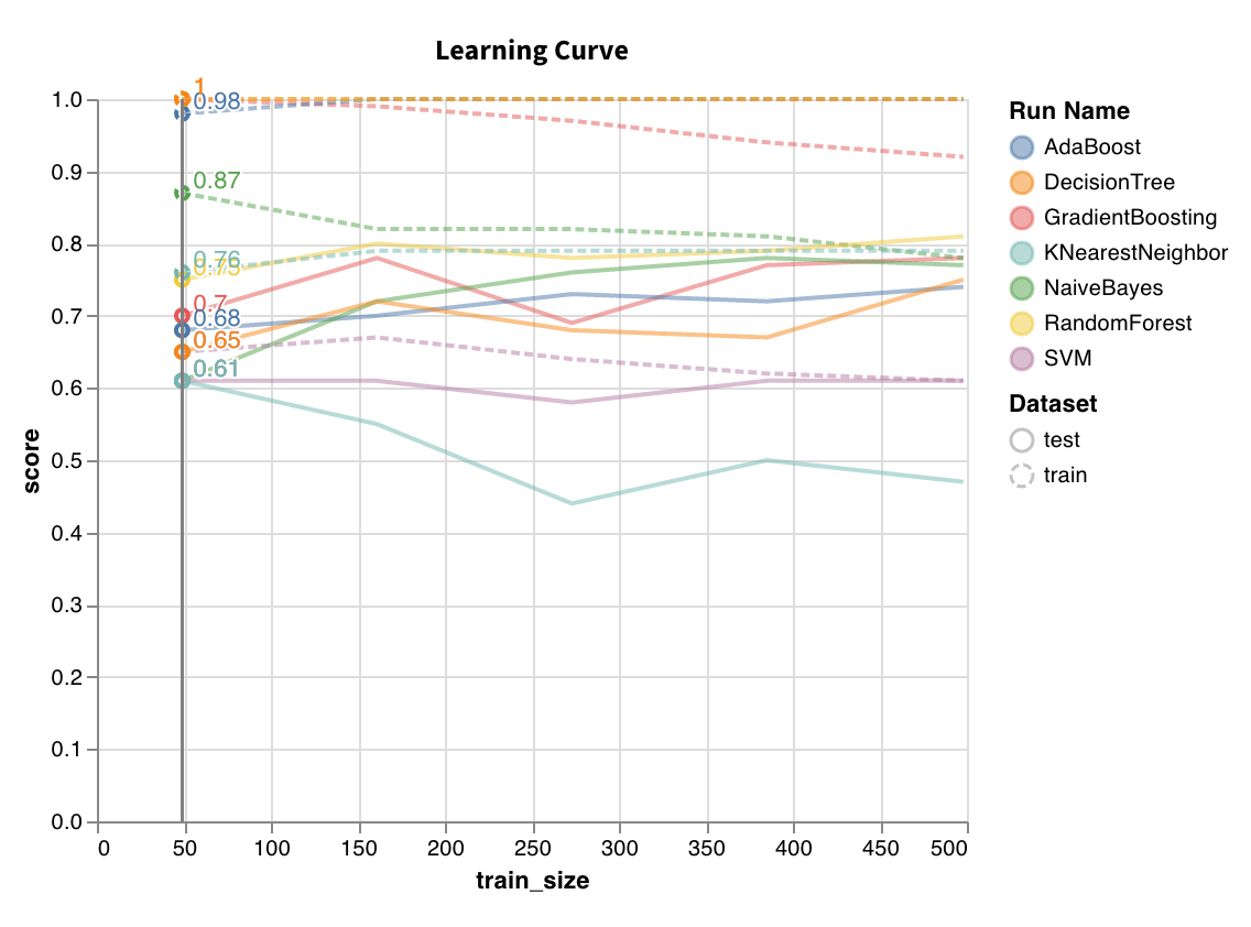 サイズの異なるデータセットでモデルをトレーニングし、トレーニングセットとテストセットの両方について、データセットサイズに対する交差検証スコアのプロットを生成します。
`wandb.sklearn.plot_learning_curve(model, X, y)`
* model (clf or reg): 学習済みの回帰モデルまたは分類器を受け取ります。
* X (arr): データセットの特徴量。
* y (arr): データセットのラベル。
サイズの異なるデータセットでモデルをトレーニングし、トレーニングセットとテストセットの両方について、データセットサイズに対する交差検証スコアのプロットを生成します。
`wandb.sklearn.plot_learning_curve(model, X, y)`
* model (clf or reg): 学習済みの回帰モデルまたは分類器を受け取ります。
* X (arr): データセットの特徴量。
* y (arr): データセットのラベル。
### ROC
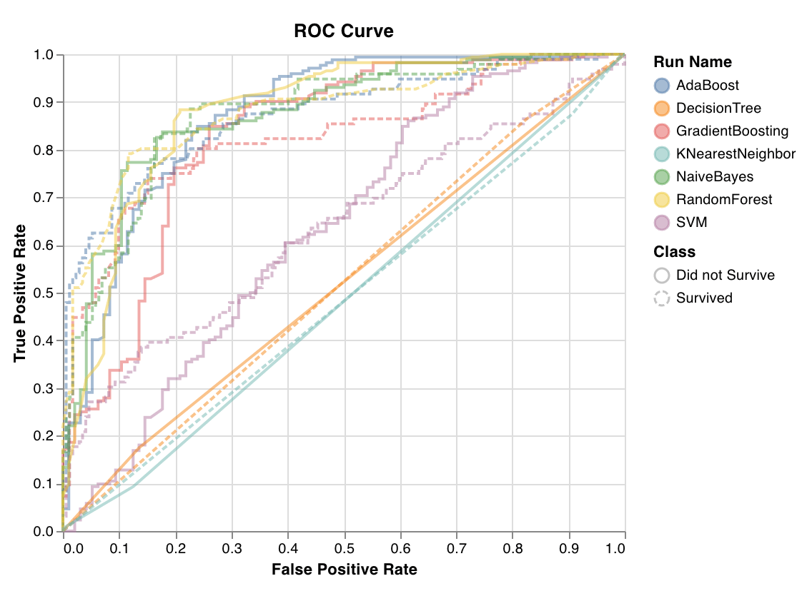 ROC曲線は、真陽性率 (y軸) と偽陽性率 (x軸) をプロットしたものです。理想的な値は TPR = 1 かつ FPR = 0 で、左上の点に相当します。通常は ROC曲線下面積 (AUC-ROC) を計算し、AUC-ROC は大きいほど優れています。
`wandb.sklearn.plot_roc(y_true, y_probas, labels)`
* y\_true (arr): テストセットのラベル。
* y\_probas (arr): テストセットの予測確率。
* labels (list): ターゲット変数 (y) のラベル名。
ROC曲線は、真陽性率 (y軸) と偽陽性率 (x軸) をプロットしたものです。理想的な値は TPR = 1 かつ FPR = 0 で、左上の点に相当します。通常は ROC曲線下面積 (AUC-ROC) を計算し、AUC-ROC は大きいほど優れています。
`wandb.sklearn.plot_roc(y_true, y_probas, labels)`
* y\_true (arr): テストセットのラベル。
* y\_probas (arr): テストセットの予測確率。
* labels (list): ターゲット変数 (y) のラベル名。
### クラスの比率
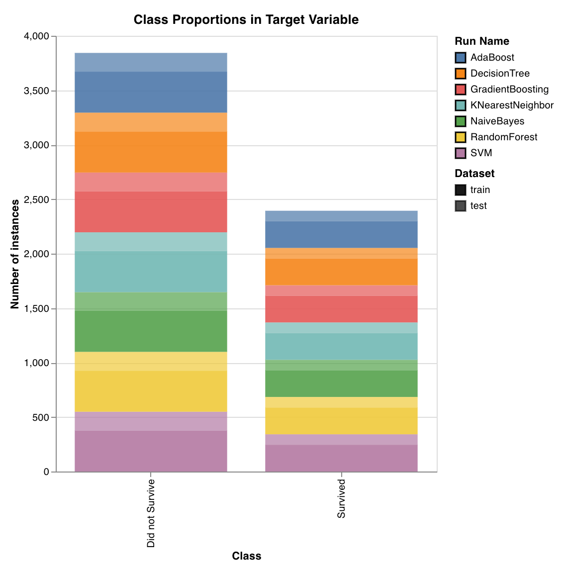 トレーニングセットとテストセットにおけるターゲットクラスの分布をプロットします。クラスの不均衡を検出し、特定のクラスがモデルに過度な影響を与えていないことを確認するのに役立ちます。
`wandb.sklearn.plot_class_proportions(y_train, y_test, ['dog', 'cat', 'owl'])`
* y\_train (arr): トレーニングセットのラベル。
* y\_test (arr): テストセットのラベル。
* labels (list): ターゲット変数 (y) のラベル名。
トレーニングセットとテストセットにおけるターゲットクラスの分布をプロットします。クラスの不均衡を検出し、特定のクラスがモデルに過度な影響を与えていないことを確認するのに役立ちます。
`wandb.sklearn.plot_class_proportions(y_train, y_test, ['dog', 'cat', 'owl'])`
* y\_train (arr): トレーニングセットのラベル。
* y\_test (arr): テストセットのラベル。
* labels (list): ターゲット変数 (y) のラベル名。
### 適合率-再現率曲線
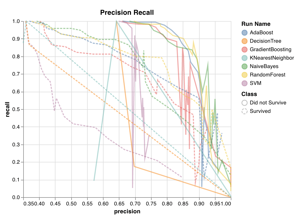 異なるしきい値における適合率と再現率のトレードオフを計算します。曲線下面積が大きいほど、再現率と適合率の両方が高いことを示します。適合率が高いことは偽陽性率が低いことを、再現率が高いことは偽陰性率が低いことを意味します。
両方のスコアが高い場合、その分類器は正確な結果を返しており (高い適合率) 、さらに陽性結果の大半を返している (高い再現率) ことを示します。PR 曲線は、クラスの不均衡が非常に大きい場合に有用です。
`wandb.sklearn.plot_precision_recall(y_true, y_probas, labels)`
* y\_true (arr): テストセットのラベル。
* y\_probas (arr): テストセットの予測確率。
* labels (list): ターゲット変数 (y) のラベル名。
異なるしきい値における適合率と再現率のトレードオフを計算します。曲線下面積が大きいほど、再現率と適合率の両方が高いことを示します。適合率が高いことは偽陽性率が低いことを、再現率が高いことは偽陰性率が低いことを意味します。
両方のスコアが高い場合、その分類器は正確な結果を返しており (高い適合率) 、さらに陽性結果の大半を返している (高い再現率) ことを示します。PR 曲線は、クラスの不均衡が非常に大きい場合に有用です。
`wandb.sklearn.plot_precision_recall(y_true, y_probas, labels)`
* y\_true (arr): テストセットのラベル。
* y\_probas (arr): テストセットの予測確率。
* labels (list): ターゲット変数 (y) のラベル名。
### 特徴量重要度
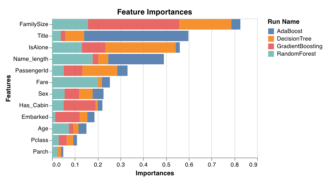 分類タスクにおける各特徴量の重要度を評価してプロットします。`feature_importances_` 属性を持つ分類器 (決定木系モデルなど) でのみ動作します。
`wandb.sklearn.plot_feature_importances(model, ['width', 'height, 'length'])`
* model (clf): 学習済みの分類器を受け取ります。
* feature\_names (list): 特徴量の名前です。特徴量のインデックスを対応する名前に置き換えることで、プロットが読みやすくなります。
分類タスクにおける各特徴量の重要度を評価してプロットします。`feature_importances_` 属性を持つ分類器 (決定木系モデルなど) でのみ動作します。
`wandb.sklearn.plot_feature_importances(model, ['width', 'height, 'length'])`
* model (clf): 学習済みの分類器を受け取ります。
* feature\_names (list): 特徴量の名前です。特徴量のインデックスを対応する名前に置き換えることで、プロットが読みやすくなります。
### キャリブレーション曲線
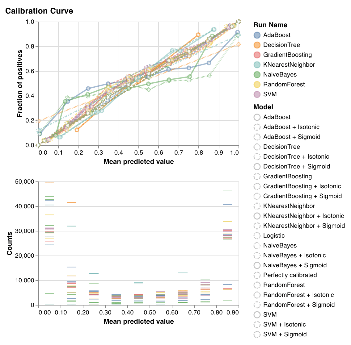 分類器の予測確率がどの程度適切にキャリブレーションされているか、また未キャリブレーションの分類器をどのようにキャリブレーションできるかをプロットします。ベースラインのロジスティック回帰モデル、引数として渡されたモデル、その等張キャリブレーションとシグモイドキャリブレーションによって推定された予測確率を比較します。
キャリブレーション曲線は、対角線に近いほど良好です。反転したシグモイド状の曲線は過学習した分類器を表し、シグモイド状の曲線は学習不足の分類器を表します。モデルの等張キャリブレーションとシグモイドキャリブレーションをトレーニングしてそれらの曲線を比較することで、モデルが過学習か学習不足か、またその場合にどのキャリブレーション (シグモイドまたは等張) が改善に役立つ可能性があるかを判断できます。
詳細については、[sklearn のドキュメント](https://scikit-learn.org/stable/auto_examples/calibration/plot_calibration_curve.html)を参照してください。
`wandb.sklearn.plot_calibration_curve(clf, X, y, 'RandomForestClassifier')`
* model (clf): 学習済みの分類器を受け取ります。
* X (arr): トレーニングセットの特徴量。
* y (arr): トレーニングセットのラベル。
* model\_name (str): モデル名。デフォルトは 'Classifier'
分類器の予測確率がどの程度適切にキャリブレーションされているか、また未キャリブレーションの分類器をどのようにキャリブレーションできるかをプロットします。ベースラインのロジスティック回帰モデル、引数として渡されたモデル、その等張キャリブレーションとシグモイドキャリブレーションによって推定された予測確率を比較します。
キャリブレーション曲線は、対角線に近いほど良好です。反転したシグモイド状の曲線は過学習した分類器を表し、シグモイド状の曲線は学習不足の分類器を表します。モデルの等張キャリブレーションとシグモイドキャリブレーションをトレーニングしてそれらの曲線を比較することで、モデルが過学習か学習不足か、またその場合にどのキャリブレーション (シグモイドまたは等張) が改善に役立つ可能性があるかを判断できます。
詳細については、[sklearn のドキュメント](https://scikit-learn.org/stable/auto_examples/calibration/plot_calibration_curve.html)を参照してください。
`wandb.sklearn.plot_calibration_curve(clf, X, y, 'RandomForestClassifier')`
* model (clf): 学習済みの分類器を受け取ります。
* X (arr): トレーニングセットの特徴量。
* y (arr): トレーニングセットのラベル。
* model\_name (str): モデル名。デフォルトは 'Classifier'
### 混同行列
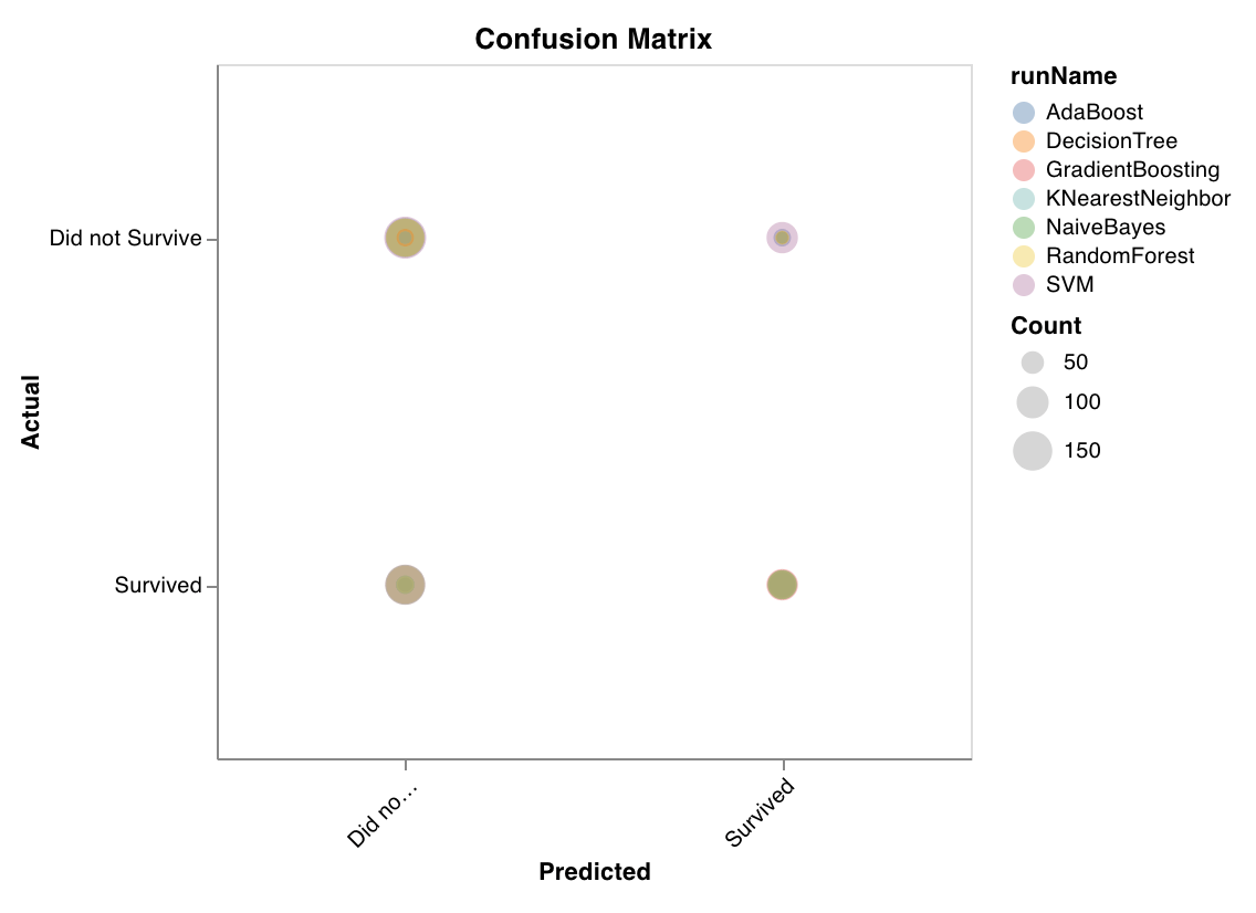 分類の精度を評価するための混同行列を計算します。これは、モデルの予測品質を評価し、モデルが誤った予測にどのようなパターンがあるかを見つけるのに役立ちます。対角線は、実際のラベルが予測ラベルと一致する場合など、モデルが正しく予測した箇所を表します。
`wandb.sklearn.plot_confusion_matrix(y_true, y_pred, labels)`
* y\_true (arr): テストセットのラベル。
* y\_pred (arr): テストセットの予測ラベル。
* labels (list): ターゲット変数 (y) のラベル名。
分類の精度を評価するための混同行列を計算します。これは、モデルの予測品質を評価し、モデルが誤った予測にどのようなパターンがあるかを見つけるのに役立ちます。対角線は、実際のラベルが予測ラベルと一致する場合など、モデルが正しく予測した箇所を表します。
`wandb.sklearn.plot_confusion_matrix(y_true, y_pred, labels)`
* y\_true (arr): テストセットのラベル。
* y\_pred (arr): テストセットの予測ラベル。
* labels (list): ターゲット変数 (y) のラベル名。
### 要約メトリクス
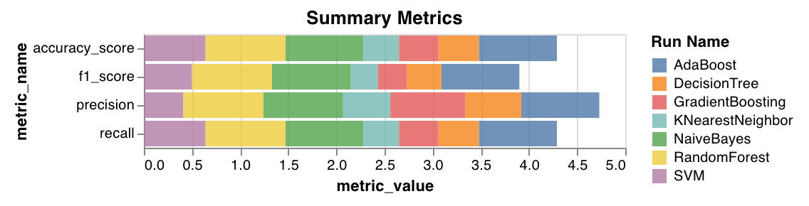 * 分類の要約メトリクスとして、`mse`、`mae`、`r2` スコアなどを計算します。
* 回帰の要約メトリクスとして、`f1`、accuracy、precision、recall などを計算します。
`wandb.sklearn.plot_summary_metrics(model, X_train, y_train, X_test, y_test)`
* model (clf or reg): 学習済みの回帰モデル または 分類器 を受け取ります。
* X (arr): トレーニングセットの特徴量。
* y (arr): トレーニングセットのラベル。
* X\_test (arr): テストセットの特徴量。
* y\_test (arr): テストセットのラベル。
* 分類の要約メトリクスとして、`mse`、`mae`、`r2` スコアなどを計算します。
* 回帰の要約メトリクスとして、`f1`、accuracy、precision、recall などを計算します。
`wandb.sklearn.plot_summary_metrics(model, X_train, y_train, X_test, y_test)`
* model (clf or reg): 学習済みの回帰モデル または 分類器 を受け取ります。
* X (arr): トレーニングセットの特徴量。
* y (arr): トレーニングセットのラベル。
* X\_test (arr): テストセットの特徴量。
* y\_test (arr): テストセットのラベル。
### エルボープロット
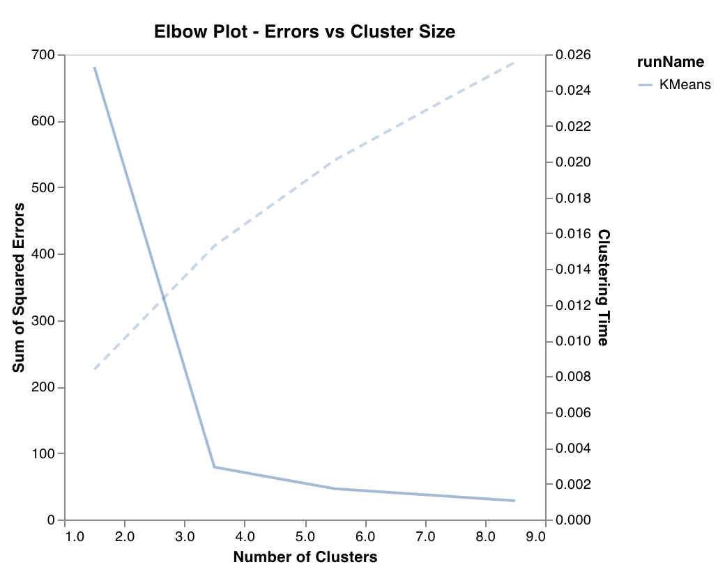 クラスタ数に応じた分散説明率を測定してプロットし、あわせてトレーニング時間も表示します。最適なクラスタ数を選ぶ際に役立ちます。
`wandb.sklearn.plot_elbow_curve(model, X_train)`
* model (clusterer): 学習済みのクラスタラーを受け取ります。
* X (arr): トレーニングセットの特徴量。
クラスタ数に応じた分散説明率を測定してプロットし、あわせてトレーニング時間も表示します。最適なクラスタ数を選ぶ際に役立ちます。
`wandb.sklearn.plot_elbow_curve(model, X_train)`
* model (clusterer): 学習済みのクラスタラーを受け取ります。
* X (arr): トレーニングセットの特徴量。
### シルエットプロット
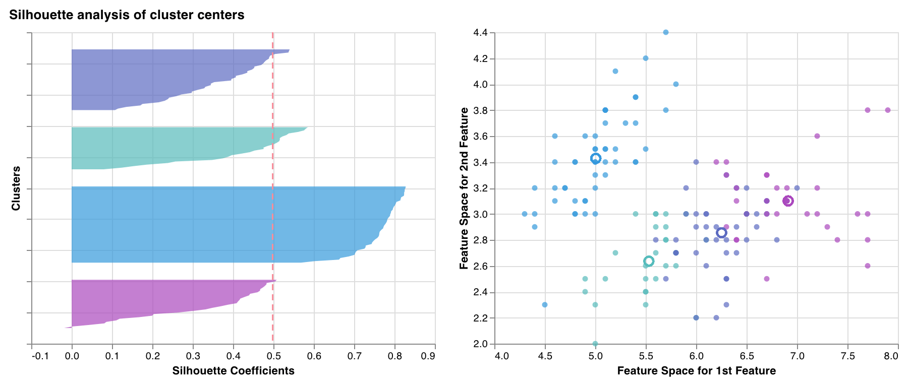 各クラスター内の各点が、隣接するクラスターの点群とどの程度近いかを測定し、プロットします。クラスターの厚みはクラスターのサイズに対応します。縦線は、すべての点の平均シルエットスコアを表します。
シルエット係数が +1 に近い場合、そのサンプルは隣接するクラスターから十分に離れていることを示します。値が 0 の場合、そのサンプルは 2 つの隣接するクラスター間の境界上、またはそのごく近くにあることを示します。負の値は、それらのサンプルが誤ったクラスターに割り当てられている可能性を示します。
一般に、すべてのクラスターのシルエットスコアは平均より上 (赤い線を超える) で、できるだけ 1 に近いことが望まれます。また、クラスターサイズもデータの根底にあるパターンを反映していることが望まれます。
`wandb.sklearn.plot_silhouette(model, X_train, ['spam', 'not spam'])`
* model (clusterer): 学習済みのクラスタラーを受け取ります。
* X (arr): トレーニングセットの特徴量。
* cluster\_labels (list): クラスターラベルの名前。クラスターのインデックスを対応する名前に置き換えることで、プロットが読みやすくなります。
各クラスター内の各点が、隣接するクラスターの点群とどの程度近いかを測定し、プロットします。クラスターの厚みはクラスターのサイズに対応します。縦線は、すべての点の平均シルエットスコアを表します。
シルエット係数が +1 に近い場合、そのサンプルは隣接するクラスターから十分に離れていることを示します。値が 0 の場合、そのサンプルは 2 つの隣接するクラスター間の境界上、またはそのごく近くにあることを示します。負の値は、それらのサンプルが誤ったクラスターに割り当てられている可能性を示します。
一般に、すべてのクラスターのシルエットスコアは平均より上 (赤い線を超える) で、できるだけ 1 に近いことが望まれます。また、クラスターサイズもデータの根底にあるパターンを反映していることが望まれます。
`wandb.sklearn.plot_silhouette(model, X_train, ['spam', 'not spam'])`
* model (clusterer): 学習済みのクラスタラーを受け取ります。
* X (arr): トレーニングセットの特徴量。
* cluster\_labels (list): クラスターラベルの名前。クラスターのインデックスを対応する名前に置き換えることで、プロットが読みやすくなります。
### 外れ値候補プロット
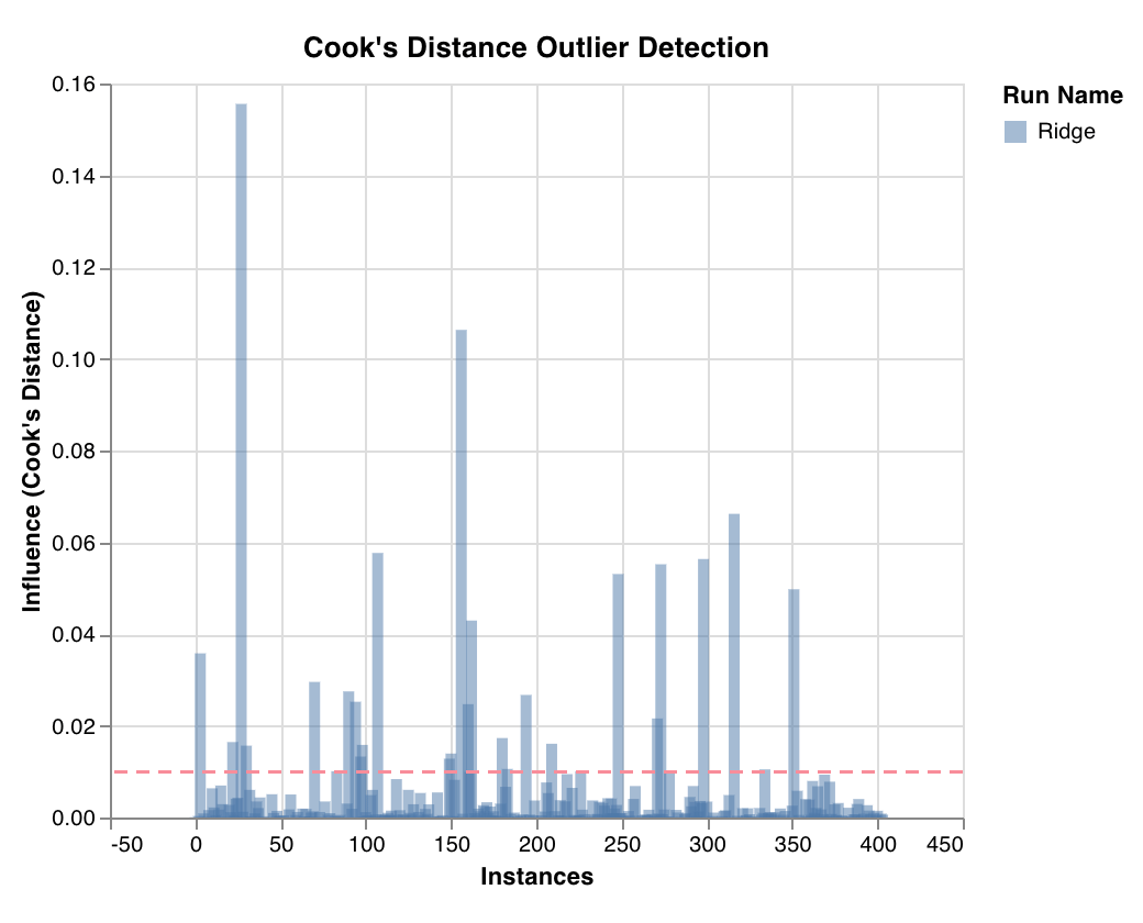 Cook's distance を用いて、データポイントが回帰モデルに与える影響を測定します。影響が大きく偏っているインスタンスは、外れ値である可能性があります。外れ値の検出に役立ちます。
`wandb.sklearn.plot_outlier_candidates(model, X, y)`
* model (regressor): 学習済みの回帰モデルを受け取ります。
* X (arr): トレーニングセットの特徴量。
* y (arr): トレーニングセットのラベル。
Cook's distance を用いて、データポイントが回帰モデルに与える影響を測定します。影響が大きく偏っているインスタンスは、外れ値である可能性があります。外れ値の検出に役立ちます。
`wandb.sklearn.plot_outlier_candidates(model, X, y)`
* model (regressor): 学習済みの回帰モデルを受け取ります。
* X (arr): トレーニングセットの特徴量。
* y (arr): トレーニングセットのラベル。
### 残差プロット
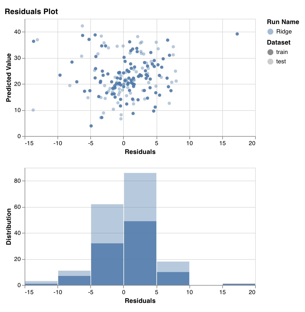 予測したターゲット値 (y軸) と、実際のターゲット値と予測値の差 (x軸) を測定してプロットし、あわせて残差誤差の分布も表示します。
一般に、適切に適合したモデルの残差はランダムに分布しているはずです。これは、優れたモデルがランダム誤差を除くデータセット内の現象の大半を捉えられるためです。
`wandb.sklearn.plot_residuals(model, X, y)`
* model (regressor): 学習済みの分類器を受け取ります。
* X (arr): トレーニングセットの特徴量。
* y (arr): トレーニングセットのラベル。
ご不明な点があれば、[Slackコミュニティ](https://wandb.me/slack) でお気軽にご質問ください。
予測したターゲット値 (y軸) と、実際のターゲット値と予測値の差 (x軸) を測定してプロットし、あわせて残差誤差の分布も表示します。
一般に、適切に適合したモデルの残差はランダムに分布しているはずです。これは、優れたモデルがランダム誤差を除くデータセット内の現象の大半を捉えられるためです。
`wandb.sklearn.plot_residuals(model, X, y)`
* model (regressor): 学習済みの分類器を受け取ります。
* X (arr): トレーニングセットの特徴量。
* y (arr): トレーニングセットのラベル。
ご不明な点があれば、[Slackコミュニティ](https://wandb.me/slack) でお気軽にご質問ください。
## 例
* [Colabで実行](https://wandb.me/scikit-colab): すぐに始められるシンプルなノートブックです。